Lunchtime learning

This is a relatively unknown and little used feature in Excel, but can be very useful where you need to compare a range of possible inputs into a calculation. There are two types of data table: a 'one-way' table that allows several alternatives for a single input to be compared, and a 'two-way' table that caters for two changing inputs.

Let's look at a simple one-way table first. We'll imagine that we want to look at projected sales figures from a range of possible starting sales values. To start with we'll enter our three data values and in cell B4 the formula that calculates the Final sales value:

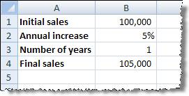
Our formula is:

=B1*(1+B2)^B3

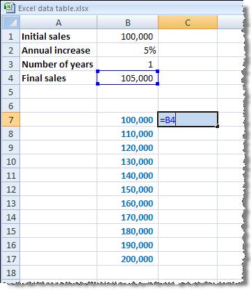
Now let's assume that we want to know what the final sales would be for different initial sales figures. We can type in a list of different starting values, and immediately to the right of the first value in our table we type a reference to our formula cell: B4:

To create our data table, select the range of cells including our list of starting values and the cells immediately to the right. Then select the option Data, Table (Excel 2007: Data ribbon, Data Tools group, What-If Analysis, Data Table):

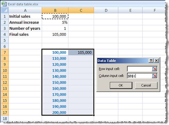
For a one-way data table where we have the list of values arranged vertically, we only need to enter the 'Column input cell' - this should be the cell that contains the value that is to be replaced in the formula with each one of the list of values. So, in our case, it is cell B1 that contains the 'Initial sales' value, and we have created a list of alternative values for B1. When we click the OK button, our table will be created:

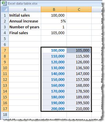
The formulae in cells C8 to C17 are created as the array formula:

{=TABLE(,B1)}

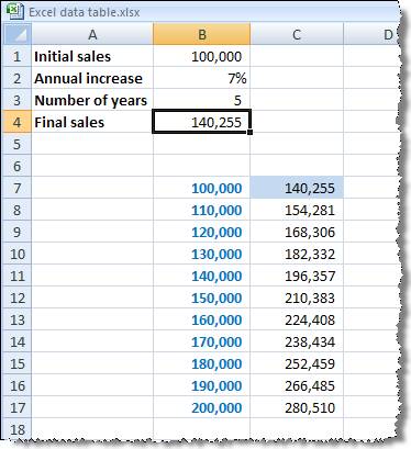
We can now change our original data values to see the results in our table. For example we can change the growth rate and number of years as follows:

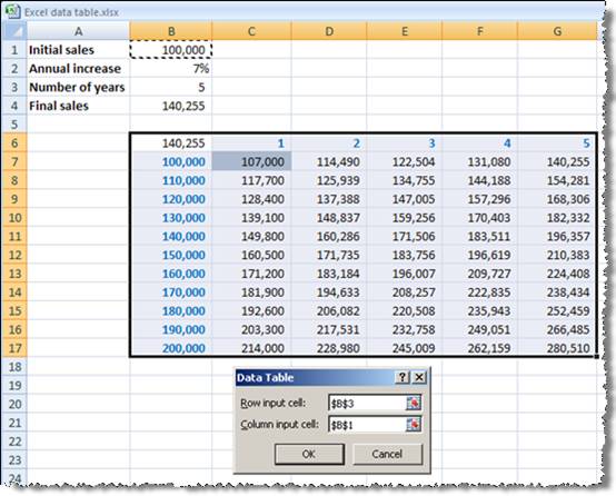
As we said earlier, we can have one-way or two-way data tables. Let's assume that in our case we want to create a table that not only shows the final sales value for different initial sales values, but also shows the different values for different numbers of years. To do this we can start with our one-way data table but instead of entering the reference to the formula to the right of the first value in our table, we enter it in the cell immediately above the first value (B6). We then enter our different numbers of years to the right of the formula cell (say C6:G6). Then select the entire table from the formula cell at the top left hand corner. Again we use the Data Table option, but this time we need to enter a 'Row input cell' as well as a 'Column input cell'.

The 'Row input cell' will refer to B3, the cell that contains our Number of years, and the 'Column input cell will continue to refer to B1: