
Lunchtime learning - Excel
 |
Use with care
Do make sure that any tips and suggestions work as you expect them to in your own particular circumstances.
Excel's Indirect function allows the creation of a formula by referring to the contents of a cell, rather than the cell reference itself. Of all the functions covered in our Excel courses, it is often Indirect() that attendees haven't come across but find an immediate use for, often saving a great deal of time and effort in the process.

If you have several sheets, each with information for a single department for example, you may want to set up a summary sheet. Rather than creating separate formulae to refer to each sheet, Indirect() can allow you to create a single set of formulae all of which use a reference to a sheet name held in a cell - hopefully an example will make this clearer.
To refer to cell A2 on a sheet named 'Cuddly Toys' we would use a formula like this:
='Cuddly toys'!A2
However, sometimes it would be useful to be able to change a whole series of references to, for example, a different sheet.
We could type the sheet name into a cell on our main sheet, say A1. We could then write a formula to refer to cell A2 on the sheet typed into cell A1.
If we simply type:
=A1!A2
Excel, not unreasonably, looks for a sheet named A1 and fails to find it.
However, we can use the Indirect function instead. Here is the screen from the Paste Function dialog for Indirect:

"'" & $A$1 & "'!A2"
Our Ref_text entry is a little confusing, so we have highlighted the pairs of speech marks in different colours. We have two items of text, and sandwiched in between them, an absolute reference to the contents of cell A1 - as you can see this correctly returns the contents of that cell - Cuddly toys. The ampersands are used to join the 3 elements of our Ref_Text together. The first text section simply holds a single apostrophe - this is necessary because, if our sheet name contains a space, it must be surrounded by apostrophes to be correctly identified. The second section contains an absolute reference to cell A1 - the cell where we type the name of our sheet. The third text section contains the closing apostrophe for the sheet name, together with the exclamation mark that separates sheet name from cell reference, and the cell reference itself - A2.
This works well to return the contents of cell A2 on our cuddly toys sheet, and if we were to type in 'Boardgames' for example, it would automatically return the contents of cell A2 on a sheet named 'Boardgames'.
However we do have a problem left to solve. We need to refer to many cells on the price list sheets, but if we copy our Indirect cell, the reference to A2 doesn't change, because it is just text. We can solve this by using a row/column style reference instead of A2:

"'" & $A$1 & "'!RC"
Note that we have to set the 'A1' argument of the function to 'False' to use this reference. RC will return the current row and column - so a formula in cell A2 will refer to A2 on cuddly toys, A3 to A3 and so on. If we need to refer to a different cell we would add numbers in square brackets after R and C. So R[1]C[1] would look at the cell one row down and one column right for example.
Get lots more Microsoft Office hints and tips
Using Excel text functions to work with analysis codes - part 1
This is the first part of a two part article that was prompted by a comparatively simple query about concatenating text. As well as dealing with that query, we'll look at some of the simpler Excel text functions for working with text. Part 2 will follow shortly and, in it, I'll look at some slightly more advanced functions for dealing with less predictable text entries.

First of all let's deal with the actual query, which asked how to combine text in two separate cells into a single cell. There are two principal ways to achieve this. Perhaps the simplest is to use the '&' within an Excel formula:

In our example we have typed three items of text in columns A, B and C. In cell D1 we have entered the following formula to combine all three into a single cell:
=A1 & " " & B1 & " " & C1
Alternatively, there is an Excel function that concatenates text in this way. Unsurprisingly it is the 'Concatenate' function.
In the following screen shot we have used 'Insert, Function' to enter the required details. Note that in order to include spaces between the items of text, we have included “ “ between each pair of cells. Using the Insert Function screen, you just need to enter a space in the appropriate text box - Excel will add the speech marks for you:

So far so good, now let's see how we cope with combining numbers and text. If we just want the number without worrying about the number format, then we can use exactly the same formula as for two items of text. Here we have included some 'literal' text in the formula together with a number in a cell:

As you can see the format is not ideal:
In the following example we have used the 'Text' function to format the number in the cell:

Note that you can also use named ranges. So if we name cell B3 as 'profit' we could write the formula as:
="Profit is " & TEXT(profit,"£#,##0")
Note that we have included a space after the 'is' and before the “ so that the number does not follow on immediately from the text.
To see the text functions available in Excel, select Insert, Function and then choose the 'Text' category (note that the examples shown are from Excel 2003, other versions' screens are slightly different):

As you can see there are lots of text functions, we will look at a few in detail, but if you want to explore all of them, just scroll through the list using the down arrow key. As you select each function in turn you will see a brief description of what it does towards the bottom of the screen. For more details, click on the 'Help on this function' link:

This group of functions can be used to return specific sets of characters from a text string. As you would imagine, Left is used to return a certain number of characters from the beginning of a text string, Right is used to return characters from the end and Mid to return characters from anywhere within the text string.
As an example, we will look at some nominal ledger codes. We will assume that the first two characters represent the company, the next three the branch, and the last four the type of expense or income:

First of all we will use the Left function to list the first two characters in the company column. We can either use Insert, Function or just type the function in directly if we know the required syntax:
=LEFT(A7,2)

Now let's use Right in a similar way to sort out the four characters from the end of the code:
=RIGHT(A7,4)

As you can see, the syntax of Left and Right are very similar, just referring to the cell holding the code and the number of characters. The final function that we will look at in this section is 'Mid' and the syntax for this one is slightly more involved because we need not only to specify the number of characters, but also from which character to start. For this reason you may find it easier to use Insert, Function:

This should create the following formula:

If we now copy the three formulae down to the end of our list, we can see how our text string has been split into the three different sections:

Get lots more Microsoft Office hints and tips
Excel - working with text functions - 2
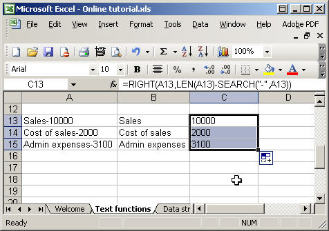
Now let's consider a slightly more difficult situation. In the following example we have a description and an amount in the same cell, but the two are always separated by a hyphen:
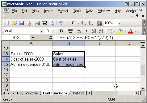
Because neither the length of the text or the figure are necessarily consistent, we can't use Left, Right or Mid. However, we can instead use the hyphen to work out where the description ends and the number begins. To do this we must first identify how many characters from the left there are before the hyphen. To do this we use the 'Search' function. Here is the function screen for Search:
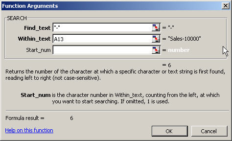
Note again that we can just type the hyphen into the 'Find_text' box and Excel will automatically add the speech marks. Note also that there is the option to specify the character position at which you want to start the search. This is useful if you need to locate more than one similar character - once you have found the first, you can start the next search from one character position higher. Our example is a simple one that doesn't use the 'Start_num' argument and, as you can see, it returns the position of the hyphen as character 6. =SEARCH("-",A13) We can now 'nest' the Search function within the 'Left' function to retrieve the description: =LEFT(A13,SEARCH("-",A13)-1) In order to exclude the hyphen itself we have subtracted 1 from the result of search. If we copy this formula down our list we can see that it achieves the desired result:
Now to deal with the amount. Whilst we can use Search to find the starting position, we don't yet know how long the amount is. We can work this out using the 'Len' function. 'Len' is a very simple function with just one argument - the text string, or cell containing the text string, that we wish to find the length of: =LEN(A13) This tells us how long the text is in total, and we have already used Search once to find the position of the hyphen. By combining Len and Search we can calculate how many characters follow the hyphen: =LEN(A13)-(SEARCH("-",A13)) In the case of “Sales-10000” Len will return 11, the hyphen is at position 6, so 11-6 = 5, the number of characters in the amount. We can use this with the 'Right' function to pick out the amount: =RIGHT(A13,LEN(A13)-(SEARCH("-",A13))) Again we can copy this formula down the list:
 As you can see above, whilst we have indeed separated out the amount characters, Excel is still treating our text as text and if we used Sum to total column C we would get zero:
We need to convert the text 'amounts' into proper numbers. To do this we use the function Value. We will use the value function to convert the three items in our list to numbers. Here is the formula for cell D13:
As you can see above, whilst we have indeed separated out the amount characters, Excel is still treating our text as text and if we used Sum to total column C we would get zero:
We need to convert the text 'amounts' into proper numbers. To do this we use the function Value. We will use the value function to convert the three items in our list to numbers. Here is the formula for cell D13:
=VALUE(C13) We can now copy this down our list and use Sum again to total our new column:
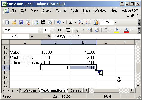
As you can see, the text values are now treated as numbers and Sum works correctly. These two functions can be used to remove unwanted characters from text. Sometimes, if you import text from other sources, you may end up with non-printing characters, such as carriage returns - Clean will remove these. Trim can be used to get rid of extraneous spaces: In the following example we have part of an address that includes multiple spaces between 'High' and 'Street' and a carriage return character to separate the lines of the address. In column B we have used Trim to get rid of the extra spaces: =TRIM(A19) and then in column C we have used Clean on the result to remove the carriage return: =CLEAN(B19)
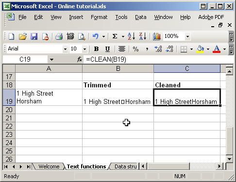
Note that the Trim function leaves a single space between High and Street, but that the Clean function removes the carriage return entirely.
Design by Reading Room Ltd 1998